By Ben Keiser, Applied Flow Technology
Creating a pump and system curve for a simple piping system with a single flow path and no control features is a relatively simple process. However, as piping systems are quite complicated with lots of branch points, control features, and dynamic interactions, creating a useful system curve can quickly become a common source of confusion. Plotting a pump and system curve for a multi-branched system can be confusing and ambiguous because there are different ways in which the system curve can be generated. Before demonstrating the system curve generation process for a multi-branched piping system, let’s review what these curves are and why they are important.
A pump and system curve plotted together is an incredibly useful tool that helps an engineer better understand pump operation in a graphical manner. If a pump’s efficiency curve is plotted together with the pump and system curve, it is evident if the pump is operating closely to the best efficiency point (BEP) or not. Figure 1 provides an example of a pump and system curve with the efficiency curve and preferred operating region (POR) points to mark 70 and 120 percent of BEP included.
The BEP is the flow rate at which the pump’s efficiency is the greatest. ANSI/API 610 11th edition (2010, ISO 13709:2009) dictates a pump’s preferred operating region (POR) to be within 70 to 120 percent of the pump’s BEP. The recommended POR of a pump dictated by ANSI/HI Standard 9.6.3-2017 can be as wide as 70 to 120 percent or as narrow as 90 to 110 percent depending on the pump’s specific speed. Overall, the goal is to operate as close to the BEP as possible.
As operation and system conditions change, the pump and system curves can intersect at different points. When the pump and system curves intersect at flow rates further away from the BEP, especially when outside the POR, various problems such as excessive vibration, suction/discharge recirculation, cavitation, low bearing/seal life, and other issues can become prevalent.
The shape of a system curve is also important to consider. A flatter system curve with a high static head is indicative of a static dominated system where the majority of the pump work is to overcome significant elevation differences in addition to frictional losses. A frictionally dominated system will typically have a steeper system curve and the pump’s primary job is to overcome significant frictional losses. For frictionally dominated systems with steeper system curves, the impact of adding more pumps in parallel operation to generate more flow will sometimes not generate significantly more flow. There is a point of diminishing return with more and more pumps. A closed system is an example of a frictionally dominated system. Understanding the shape of the system curve is helpful to ensure that the proper pump is installed for the appropriate system it supplies.
Sometimes, multiple system curves exist when a single system curve does not uniquely represent the overall resistance. A multi-branched system is an example where this is the case.
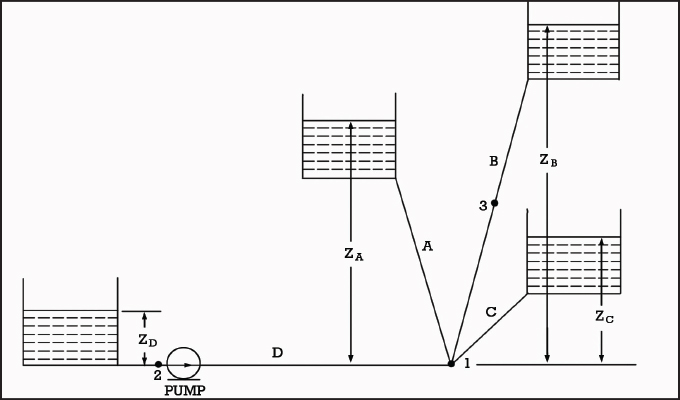
In the “Pump Handbook,” Third Edition by Karassik, Messina, Cooper, and Heald, Section 8.2 discusses Branch-Line Pumping Systems. There is a discussion on how to generate a system curve for an open-ended pumping system with multiple branch lines, such as the one shown in figure 2. J.P. Messina outlines how to develop a system curve for a network such is this by considering the individual flow paths separately.
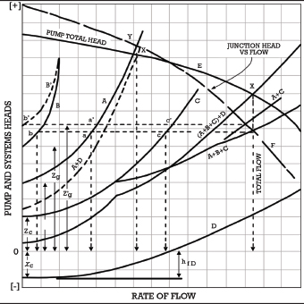
Often, multiple system curves exist for a single system, especially ones with multiple flow paths. The system curve we care about is a cumulative curve made up of the individual system curves. Figure 3 illustrates several system curves for the multi-branched network in figure 2.
Which curve best represents the entire system resistance? It depends on the reference point you are using to generate the curve. The system resistance at the pump location is different than the system resistance at the branch point where the flow splits. If you look carefully, the system curve at the branch point is represented by curve “F”, which accounts for the pump total head in figure 3. The most practical place to generate a system curve to represent the overall system resistance is at the location of a pump because this will show the frictional resistance and elevation change a pump must overcome to supply a given flow.
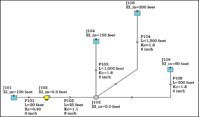
Here’s a point of complexity and confusion for creating a system curve for a network like in figure 2. Should reverse flow into the system be allowed when generating the curve? Messina mentions that forward flow into the reservoirs should not be assumed. There is a limiting elevation for the reservoirs such that they could potentially supply the system instead. Different overall system curves exist depending on if reverse flow is allowed or not. This will also impact the static head that a pump needs to overcome at zero flow. This can be easily demonstrated with a flow analysis software tool like –––Let’s consider the multi-branched piping system seen in figure 4, which is like that from the Pump Handbook. Each reservoir is at a different elevation with piping of different lengths. Each pipe includes minor losses from fittings represented with an additional K factor (Kc).
Figure 5 is the pump and system curve for the system in figure 4, generated by AFT Fathom. Also included is the efficiency curve and the Preferred Operating Range (POR) data points as dictated by ANSI/HI 9.6.3-2017. The pump operates at about 5,000 gallons per minute, which is the original design flow rate for this piping system. This is about 111 percent of BEP.
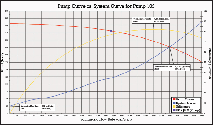
It is important to point out that there is nothing preventing reverse flow in the branch pipes. Therefore, as system curve is generated, discharge reservoirs J104 and J105 will supply flow into the system through pipes P103 and P104 at low flow rates. How can you see that this is the case? By fixing a near zero flow rate through the pump, then calculate the resulting flow rates in the pipes and you will potentially see a negative flow rate indicating reverse flow.
A LOOK AHEAD
What is the static head for a multi-branched system? This is the source of confusion and ambiguity because the static head depends on the allowance of reverse flow when generating the system curve. In the next month’s installment of this article, we’ll examine this in greater detail.
FOR MORE INFORMATION
Ben Keiser is technical sales consultant at Applied Flow Technology. He holds a bachelor’s of science in chemical engineering (2009) from the Colorado School of Mines. He can be found teaching many of AFT’s technical seminars and stopping over for lunch and learns with AFT customers. Founded in 1993, Applied Flow Technology has grown to be a leader in the pipe flow modeling software market. With a primary focus on developing high quality fluid flow analysis software, AFT has a comprehensive line of products for the analysis and design of piping and ducting systems. For more information, visit www.aft.com.
MODERN PUMPING TODAY, March 2020
Did you enjoy this article?
Subscribe to the FREE Digital Edition of Modern Pumping Today Magazine!